In this example we show how to do portfolio optimization using CVXPY. We begin with the basic definitions. In portfolio optimization we have some amount of money to invest in any of $n$ different assets. We choose what fraction $w_i$ of our money to invest in each asset $i$, $i=1, \ldots, n$.
We call $w\in {\bf R}^n$ the portfolio allocation vector. We of course have the constraint that ${\mathbf 1}^T w =1$. The allocation $w_i<0$ means a short position in asset $i$, or that we borrow shares to sell now that we must replace later. The allocation $w \geq 0$ is a long only portfolio. The quantity $ ||w||_1 = {\bf 1}^T w_+ + {\bf 1}^T w_- $ is known as leverage.
We will only model investments held for one period. The initial prices are $p_i > 0$. The end of period prices are $p_i^+ >0$. The asset (fractional) returns are $r_i = (p_i^+-p_i)/p_i$. The porfolio (fractional) return is $R = r^Tw$.
A common model is that $r$ is a random variable with mean ${\bf E}r = \mu$ and covariance ${\bf E{(r-\mu)(r-\mu)^T}} = \Sigma$. It follows that $R$ is a random variable with ${\bf E}R = \mu^T w$ and ${\bf var}(R) = w^T\Sigma w$. ${\bf E}R$ is the (mean) return of the portfolio. ${\bf var}(R)$ is the risk of the portfolio. (Risk is also sometimes given as ${\bf std}(R) = \sqrt{{\bf var}(R)}$.)
Portfolio optimization has two competing objectives: high return and low risk.
Classical (Markowitz) portfolio optimization solves the optimization problem
\begin{array}{ll} \mbox{maximize} & \mu^T w - \gamma w^T\Sigma w\\ \mbox{subject to} & {\bf 1}^T w = 1, \quad w \in {\cal W}, \end{array}
where $w \in {\bf R}^n$ is the optimization variable, $\cal W$ is a set of allowed portfolios (e.g., ${\cal W} = {\bf R}_+^n$ for a long only portfolio), and $\gamma >0$ is the risk aversion parameter.
The objective $\mu^Tw - \gamma w^T\Sigma w$ is the risk-adjusted return. Varying $\gamma$ gives the optimal risk-return trade-off. We can get the same risk-return trade-off by fixing return and minimizing risk.
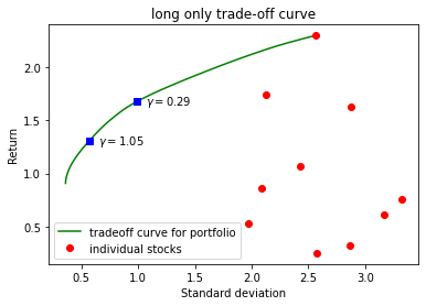
In the following example we compute and plot the optimal risk-return trade-off for fictional $10$ assets, restricting ourselves to a long only portfolio.
The input values of these assets - covariance matrix $\Sigma$ and mean values vector $\mu$ are read from the input files, the files can be chosen in the Control window. The risk aversion parameter $\gamma$ here is the logarithmic sequence in some range. For the estimates you can choose two indexes (marker # 1 and marker # 2) from this array in the Control window. Some statistics for these two values will be shown in the plots and in the console output.
The optimal risk-return trade-off for $10$ assets, restricting ourselves to a long only portfolio.
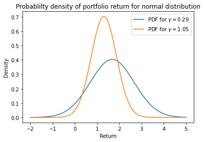
Plot of the return distributions for the two risk aversion values marked on the trade-off curve. Notice that the probability of a loss is near 0 for the low risk value and far above 0 for the high risk value.